Year-Effect
Are multiple season data comparable?

Team PC Plot
To explore whether clustering effects exist, we created the function team_pc_plot(), which first uses principal component analysis (PCA) to reduce our higher dimensional data with a larger set of variables to a smaller set of just two principal components (PCs) that still manages to retain most of the information in the original data. The new coordinate system and transformed data defined in terms of the two PCs are shown. Concentration ellipses are then used to encircle data of all teams from the same season. From the graph, we can see that data for separate years are closely packed together and there is no clear pattern of a year-effect.

Season Distance Plot
We also visualized the distance between every pair of seasons with a season distance matrix. We can see from the matrix that the closer together two years are, the smaller the in-between distance is, which is in line with our intuition.

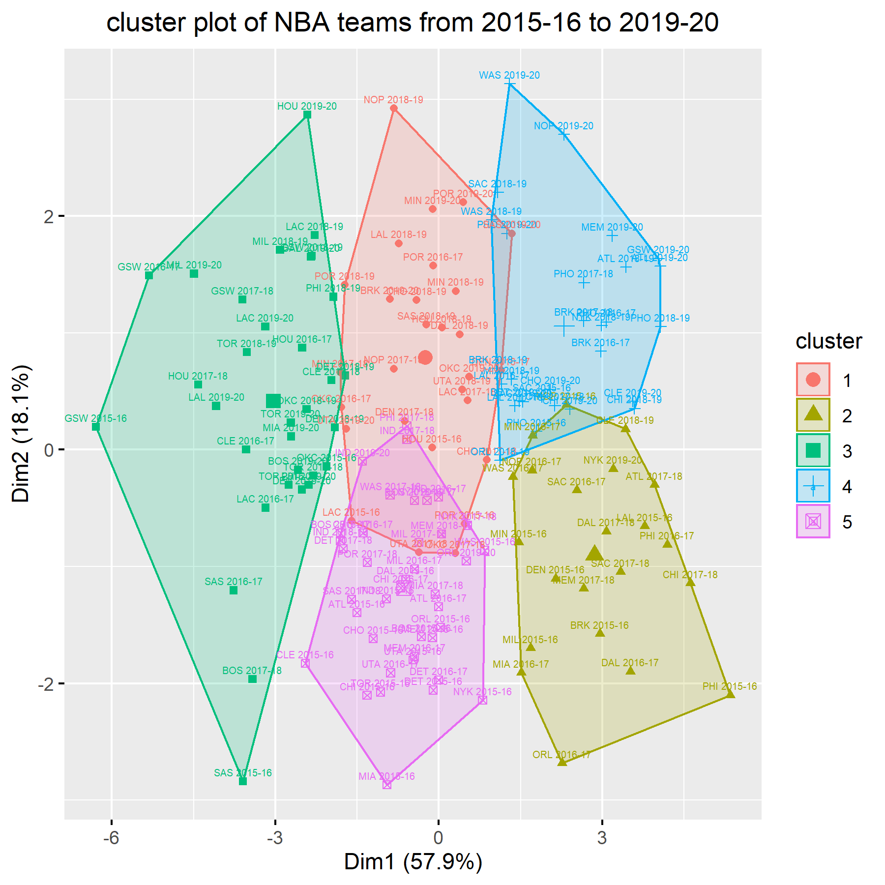
Team Cluster Plot
We created another function team_cluster_plot() that uses K-means clustering to group teams from multiple seasons into 5 clusters. The choice of 5 was based on the fact that we have data from 5 NBA seasons. We see that the algorithm results in clusters where observations from the same season are not necessarily grouped together in the same cluster. Instead, it seems that teams are clustered together based on how strong they are. For example, teams in the olive cluster are among the most competitive teams (e.g. GSW 2015-16), while teams in the blue cluster are among the least competitive teams (e.g. PHI 2015-16). Thus, again, it seems that season/year patterns are not apparent.
Integrative Prediction Using Multiple Season Data
Suppose we have multiple data sources $$\mathcal{D}_{i} = \{(x_{i1},y_{i1})...(x_{iN},y_{iN}) \} \ \ \text{for} \ i=1,...,m$$ We train $m$ separate classifiers $g_i: x_i \to y_i$, here $g$ returns the probability instead of binary outcome. When given a new sample $x$ from season $k$, we perform the weighted prediction: $$ \hat{p} = \sum_{i=1}^m w_i(k) g_i(x) $$ The weight is determined by the distance between two seasons. For season $i$ and season $j$, define the distance $d(i,j)$ from the above dimension reduction procedures, then the weight is calculated as $$ w_i(k) = \frac{1/d(i,k)}{\sum_{i=1}^m 1/d(i,k)} $$
Wrap-up Function
win_prob_prediction(train_year = c(2016:2019),test_year = 2020,year_effect = 1)